●Train Set
- 모델의 학습만 을 위해 사용
- parameter 나 feature 등을 수정하여 모델의 성능을 높이는 작업에 사용
● Test Set
- 최종적으로 모델의 성능 평가
- 실사용 되었을 때 모델이 얼마나 좋은 성능을 보일 수 있을지 알아보는 것
● Validation Set
- 모델의 학습에 직간접적으로 관여하지 않음
- 학습이 끝난 모델에 적용, 최종적으로 모델을 fine tuning하는데 사용한다
● 회귀분석과 분류분석
 |
 |
| 회귀분석 (Regression) | 분류분석 (Classfication) |
| 연속된 값을 예측 | 종류를 예측 |
| ex) 과거의 주가를 토대로 미래 주가 예측 자동차 배기량 , 연식 등 중고차 정보 이용해 가격을 예측 |
클래스 0 또는 1 중에서 선택하는 이진 분류 3개 이상의 클래스 중 하나를 선택하는 다중분류 ex) 강아지 or 고양이 |
| 선형회귀 / 랜덤 포레스트 / 그래디언트 부스팅 | 이진분류/ 다중분류 / 로지스틱 회귀 |

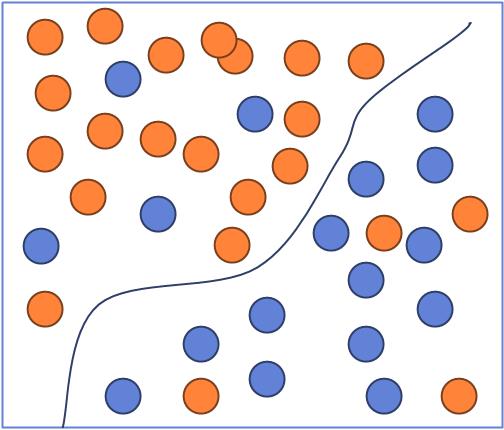
● 이진 분류
- True or False 판별하기 때문에 출력값은 오직 하나
- 출력값을 sigmoid 함수를 이용해 0과 1로 가공한다
- 직선보다 적절한 곡선을 통해 분류
- 로지스틱 회귀는 이진분류 모델을 분석하기 좋은 모델
● 다중 분류
- 다중 분류모델은 타겟의 종류가 여러개 -> 출력값도 여러개
- softmax 함수를 사용하여 0과 1사이 값으로 가공
- one-hot-encoding 이라는 기법을 사용
♣ 손실 함수
●이진 분류- binary_crossentropy(이항교차 엔트로피)
- y값이 0과 1인 이진 분류기를 훈련할 때 자주 사용되는 손실 함수
- 활성화 함수(activation) : sigmoid 사용 (출력값이 0과 1사이의 값)
● 다중 분류- categorical_crossentropy (범주형 교차 엔트로피)
- Y 클래스가 3개 이상일 경우, 즉 다중 분류에서 사용
- 활성화 함수(activation) : softmax 사용 (모든 벡터 요소의 값은 0 과 1사이의 값이 나오고, 모든 합이 1이 됨)
- 라벨이 (0,0,1,0,0) , (0,1,0,0,0) 과 같이 one-hot encoding 된 형 태로 제공될 때 사용 가능
● 다중 분류- sparse_categorical_crossentropy
- categorical crossentropy와 같이 다중 분류에서 사용
- one-hot encoding 된 상태일 필요 없이 정수 인코딩 된 상태에서 수행 가능
- 라벨이 (1,2,3,4) 와 같이 정수형태로 사용
●categorical_crossentropy/ sparse_categorical_crossentropy 의 차이점
: one-hot encoding의 자동화 여부
● 평균 제곱 오차 손실 (means squared error, MSE)
- 회귀 문제에서 널리 사용됨 회귀문제에 사용될 수 있는 다른 손실 함수
(1) 평균 절댓값 오차 (Mean absolute error, MAE)
(2) 평균 제곱근 오차(Root mean squared error, RMSE)-예측값과 실제값의 차이를 제곱하여 평균한 값(모두 실숫값 계산)
MSE가 크다는 것은 평균 사이에 차이가 크다는 뜻 /
MSE가 작다는 것 은 데이터와 평균사이의 차이가 작다는 뜻
● MSE 와 MAE의 차이
ex) 데이터 크기가 10, 10, 10, 10, 10, 10,2500,10,10,10 일때
mse(평균 제곱 오차) 는 오차가 크게 적용된다 : 이상치에 더 민감
-> 2500을 최대한 반영
mae(평균 절대 오차) 는 오차를 변수들간의 오차가 완화된다 :이상치에 덜 민감
->2500을 최소한 반영
● 결정 계수 R2 Score
-R-squared는 선형 회귀 모델에 대한 적합도 측정값이다.
-선형 회귀 모델을 훈련한 후, 모델이 데이터에 얼마나 적합한지 확인하는 통계 방법 중 하나
- r2 score는 0과 1 사이의 값을 가지며, 1에 가까울수록 선형회귀 모델이 데이터에 대해 높은 연관성을
갖는다고 해석한다
●One Hot Encoding
- 범주형 데이터를 이진 형태의 백터로 변환하는 방법
-각 범주에 대해 고유한 이진 벡터를 생성, 해당 범주에 해당하는 원소는1, 나머지 원소는 0으로 표현
-이를 통해 범주형 데이터를 머신러닝 알고리즘이 처리할 수 있는 형태로 변환 가능
ex)
| 품종 | setosa | virginica | versicolor | |
| setosa | 1 | 0 | 0 | |
| virginica | 0 | 1 | 0 | |
| versicolor | 0 | 0 | 1 | |
| setosa | 1 | 0 | 0 |
●난수값 ( random_state)
- 머신러닝 알고리즘 및 데이터 분할 작업에서 사용되는 난수 생성기의 시드 값\
- random_state 설정 시 무작위로 생성되는 난수 패턴이 고정, 알고리즘 결과의 재현을 가능하게 함
●코드실습
# train_test_split01
import numpy as np
from keras.models import Sequential
from keras.layers import Dense

# 1. 데이터
x = np.array([1, 2, 3, 4, 5, 6, 7, 8, 9, 10, 11, 12, 13, 14, 15, 16, 17, 18, 19, 20])
y = np.array([1, 2, 3, 4, 5, 6, 7, 8, 9, 10, 11, 12, 13, 14, 15, 16, 17, 18, 19, 20])
# x = np.array(range(1, 21))
# y = np.array(range(1, 21))

# print(x.shape)
# print(y.shape)
# print(x)
x_train = np.array([1, 2, 3, 4, 5, 6, 7, 8, 9, 10, 11, 12, 13, 14])
y_train = np.array([1, 2, 3, 4, 5, 6, 7, 8, 9, 10, 11, 12, 13, 14])

x_test = np.array([15, 16, 17, 18, 19, 20])
y_test = np.array([15, 16, 17, 18, 19, 20])

# 2. 모델구성
model = Sequential()
model.add(Dense(14, input_dim=1))
model.add(Dense(50))
model.add(Dense(1))

# 3. 컴파일, 훈련
model.compile(loss='mse', optimizer='adam')
model.fit(x_train, y_train, epochs=100, batch_size=1)

# 4. 평가, 예측
loss = model.evaluate(x_test, y_test)
print('loss : ', loss)

result = model.predict([21])
print('21의 예측값 : ', result)
#train_test_split
import numpy as np
from keras.models import Sequential
from keras.layers import Dense
from sklearn.model_selection import train_test_split

# 1. 데이터
x = np.array([1, 2, 3, 4, 5, 6, 7, 8, 9, 10, 11, 12, 13, 14, 15, 16, 17, 18, 19, 20])
y = np.array([1, 2, 3, 4, 5, 6, 7, 8, 9, 10, 11, 12, 13, 14, 15, 16, 17, 18, 19, 20])

x_train, x_test, y_train, y_test = train_test_split(
    x, y,           # x, y 데이터
    test_size=0.3,  # test의 사이즈 보통 30%
    train_size=0.7, # train의 사이즈는 보통 70%임
    random_state=100,  # 데이터를 난수값에 의해 추출한다는 의미, 중요한 하이퍼파라미터
    shuffle=True    # 데이터를 섞어서 가지고 올 것인지를 True/False 로 정함
)

# 2. 모델구성
model = Sequential()
model.add(Dense(14, input_dim=1))
model.add(Dense(50))
model.add(Dense(1))

# 3. 컴파일, 훈련
model.compile(loss='mse', optimizer='adam')
model.fit(x_train, y_train, epochs=100, batch_size=1)

# 4. 평가, 예측
loss = model.evaluate(x_test, y_test)
print('loss : ', loss)

result = model.predict([21])
print('21의 예측값 : ', result)
#scatter 산점도 그리기
import numpy as np
from keras.models import Sequential
from keras.layers import Dense
from sklearn.model_selection import train_test_split

# 1. 데이터
x = np.array([1, 2, 3, 4, 5, 6, 7, 8, 9, 10, 11, 12, 13, 14, 15, 16, 17, 18, 19, 20])
y = np.array([1, 2, 3, 4, 5, 6, 7, 8, 9, 10, 11, 12, 13, 14, 15, 16, 17, 18, 19, 20])

x_train, x_test, y_train, y_test = train_test_split(
    x, y,           # x, y 데이터
    test_size=0.3,  # test의 사이즈 보통 30%
    train_size=0.7, # train의 사이즈는 보통 70%임
    random_state=100,  # 데이터를 난수값에 의해 추출한다는 의미이며, 중요한 하이퍼파라미터임
    shuffle=True    # 데이터를 섞어서 가지고 올 것인지를 정함
)

# 2. 모델구성
model = Sequential()
model.add(Dense(14, input_dim=1))
model.add(Dense(50))
model.add(Dense(1))

# 3. 컴파일, 훈련
model.compile(loss='mse', optimizer='adam')
model.fit(x_train, y_train, epochs=100, batch_size=1)

# 4. 평가, 예측
loss = model.evaluate(x_test, y_test)
print('loss : ', loss)

y_predict = model.predict(x)

##### scatter 시각화
import matplotlib.pyplot as plt

plt.scatter(x, y)  # 산점도 그리기
plt.plot(x, y_predict, color='red')
plt.show()
# r2 안좋은 예 만들기
#1. R2 를 음수가 아닌 0.5 이하로
#2. 데이터는 조작 x
#3. 레이어는 인풋, 아웃풋 포함 7개 이상(히든레이어 5개 이상)으로 만들기
#4. batch_size=1
#5. 히든레이어의 노드(뉴런) 갯수는 10개 이상 100개 이하
#6. train_size = 0.7
#7. epochs=100 이상

import numpy as np
from keras.models import Sequential
from keras.layers import Dense
from sklearn.model_selection import train_test_split


#1. 데이터
x = np.array([1,2,3,4,5,6,7,8,9,10,11,12,13,14,15,16,17,18,19,20])
y = np.array([1,2,4,3,5,7,9,3,8,12,13,8,14,15,9,16,17,23,18,20])

x_train, x_test, y_train, y_test = train_test_split(
    x, y, train_size=0.7, shuffle=True, random_state=0
)
#shuffle=False 일때 0.5441042097346507

#2. 모델구성
model = Sequential()
model.add(Dense(5, input_dim=1))
model.add(Dense(10))
model.add(Dense(50))
model.add(Dense(100))
model.add(Dense(100))
model.add(Dense(100))
model.add(Dense(100))
model.add(Dense(100))
model.add(Dense(100))
model.add(Dense(100))
model.add(Dense(100))
model.add(Dense(100))
model.add(Dense(100))
model.add(Dense(100))
model.add(Dense(100))
model.add(Dense(100))
model.add(Dense(100))
model.add(Dense(100))
model.add(Dense(100))
model.add(Dense(100))
model.add(Dense(100))
model.add(Dense(100))
model.add(Dense(100))
model.add(Dense(100))
model.add(Dense(100))
model.add(Dense(100))
model.add(Dense(1))

#3. 훈련
model.compile(loss='mse', optimizer='adam')   # ==> 회귀모델
model.fit(x_train, y_train, epochs=100, batch_size=1)

#4. 평가, 예측
loss = model.evaluate(x_test, y_test)
print('loss : ', loss)

y_predict = model.predict(x)

from sklearn.metrics import r2_score
r2 = r2_score(y, y_predict)
print('r2 스코어: ', r2)


# result
# loss :  39.7522087097168
# r2 스코어:  0.49266916260562
# 노드수를 늘리고 히든레이어의 갯수를 늘리면 r2 score 가 좋지 않음
# r2score
import numpy as np
from keras.models import Sequential
from keras.layers import Dense
from sklearn.model_selection import train_test_split

# 1. 데이터
x = np.array([1, 2, 3, 4, 5, 6, 7, 8, 9, 10, 11, 12, 13, 14, 15, 16, 17, 18, 19, 20])
y = np.array([1, 2, 3, 4, 5, 6, 7, 8, 9, 10, 11, 12, 13, 14, 15, 16, 17, 18, 19, 20])

x_train, x_test, y_train, y_test = train_test_split(
    x, y,           # x, y 데이터
    test_size=0.3,  # test의 사이즈 보통 30%
    train_size=0.7, # train의 사이즈는 보통 70%임
    random_state=100,  # 데이터를 난수값에 의해 추출한다는 의미이며, 중요한 하이퍼파라미터임
    shuffle=True    # 데이터를 섞어 가져올 것인지 TRUE/FALSE로 정함
)

# 2. 모델구성
model = Sequential()
model.add(Dense(14, input_dim=1))
model.add(Dense(50))
model.add(Dense(1))

# 3. 컴파일, 훈련
model.compile(loss='mse', optimizer='adam')
model.fit(x_train, y_train, epochs=100, batch_size=1)

# 4. 평가, 예측
loss = model.evaluate(x_test, y_test)
print('loss : ', loss)

y_predict = model.predict(x)

### R2score
from sklearn.metrics import r2_score, accuracy_score
r2 = r2_score(y, y_predict)
print('r2스코어 : ', r2)

# result(1)
# loss :  3.037989699805621e-07
# r2스코어 :  0.9999999942704495

#result(2)
#loss: 2.659254278114531e-06
#r2스코어: 0.9999999507534805
#california
import numpy as np
from keras.models import Sequential
from keras.layers import Dense
from sklearn.model_selection import train_test_split
from sklearn.metrics import r2_score
# from sklearn.datasets import load_boston # 윤리적 문제로 제공안됨
from sklearn.datasets import fetch_california_housing
#1.데이터
# datasets = load_boston()
datasets = fetch_california_housing()
x = datasets.data
y = datasets.target
print(datasets.feature_names)
print(datasets.DESCR)
print(x.shape) # (20640, 8)
print(y.shape) # (20640,)
x_train, x_test, y_train, y_test = train_test_split(
x, y, train_size=0.7, random_state=72, shuffle=True
)
print(x_train.shape) # (14447, 8)
print(y_train.shape) # (14447,)
#2. 모델구성
model = Sequential()
model.add(Dense(100, input_dim=8))
model.add(Dense(100))
model.add(Dense(100))
model.add(Dense(100))
model.add(Dense(1))
#3. 컴파일, 훈련
model.compile(loss='mse', optimizer='adam')
model.fit(x_train, y_train, epochs=500, batch_size=200)
#4. 평가, 예측
loss = model.evaluate(x_test, y_test)
print('loss : ', loss)
y_predict = model.predict(x_test)
r2 = r2_score(y_test, y_predict)
print('r2 스코어 : ', r2)
# [실습] activation  함수를 사용하여 성능 향상시키기
# activation='relu'

import numpy as np
from keras.models import Sequential
from keras.layers import Dense
from sklearn.model_selection import train_test_split
from sklearn.metrics import r2_score
# from sklearn.datasets import load_boston # 윤리적 문제로 제공안됨
from sklearn.datasets import fetch_california_housing


#1.데이터
# datasets = load_boston()
datasets = fetch_california_housing()
x = datasets.data
y = datasets.target

print(datasets.feature_names)
print(datasets.DESCR)

print(x.shape)  # (20640, 8)
print(y.shape)  # (20640,)

x_train, x_test, y_train, y_test = train_test_split(
    x, y, train_size=0.7, random_state=72, shuffle=True
)
print(x_train.shape)    # (14447, 8)
print(y_train.shape)    # (14447,)

#2. 모델구성
model = Sequential()
model.add(Dense(100, activation='linear', input_dim=8))
model.add(Dense(100, activation='relu'))
model.add(Dense(100, activation='relu'))
model.add(Dense(100, activation='relu'))
model.add(Dense(1, activation='linear'))    # 회귀모델에서 인풋과 아웃풋 활성화함수는 'linear'

#3. 컴파일, 훈련
model.compile(loss='mse', optimizer='adam')
model.fit(x_train, y_train, epochs=100, batch_size=200)

#4. 평가, 예측
loss = model.evaluate(x_test, y_test)
print('loss : ', loss)

y_predict = model.predict(x_test)

r2 = r2_score(y_test, y_predict)
print('r2 스코어 : ', r2)

# result
# r2 스코어 :  0.6534469383279615
# 모든 히든레이어에 activation='relu'를 사용하면 성능이 향상됨
#cancer_sigmoid
import numpy as np
from keras.models import Sequential
from keras.layers import Dense
from sklearn.model_selection import train_test_split
from sklearn.metrics import r2_score, accuracy_score
from sklearn.datasets import load_breast_cancer
import time

#1. 데이터
datasets = load_breast_cancer()
print(datasets.DESCR)
print(datasets.feature_names)
# ['mean radius' 'mean texture' 'mean perimeter' 'mean area'
#  'mean smoothness' 'mean compactness' 'mean concavity'
#  'mean concave points' 'mean symmetry' 'mean fractal dimension'
#  'radius error' 'texture error' 'perimeter error' 'area error'
#  'smoothness error' 'compactness error' 'concavity error'
#  'concave points error' 'symmetry error' 'fractal dimension error'
#  'worst radius' 'worst texture' 'worst perimeter'' ractal dimension']
x = datasets.data
y = datasets.target
print(x.shape, y.shape) # (569, 30) (569,)

x_train, x_test, y_train, y_test = train_test_split(
    x, y, train_size=0.7, random_state=100, shuffle=True
)

#2. 모델구성
model = Sequential()
model.add(Dense(100, input_dim=30))
model.add(Dense(100))
model.add(Dense(50))
model.add(Dense(1, activation='sigmoid')) # 이진분류는 모조건 아웃풋 레이어의
                                          # 활성화 함수를 'sigmoid'로 해줘야 한다

#3. 컴파일, 훈련
model.compile(loss='binary_crossentropy', optimizer='adam',
              metrics=['accuracy','mse'])

start_time = time.time()
model.fit(x_train, y_train, epochs=100, batch_size=200, verbose=2)
end_time = time.time() - start_time

#4. 평가, 예측
# loss = model.evaluate(x_test, y_test)
loss, acc, mse = model.evaluate(x_test, y_test)
y_predict = model.predict(x_test)
print(y_predict)
print('loss : ', loss)
print('acc :', acc)
print('mse : ', mse)

# [실습] accuracy_score를 출력하라!!!
# y_predict 반올림하기

# y_predict = np.where(y_predict > 0.5, 1, 0)
y_predict = np.round(y_predict)
acc_test = accuracy_score(y_test, y_predict)
print('loss : ', loss)
print('acc : ', acc)
print('걸린 시간 : ', end_time)

# loss :  [0.25783923268318176, 0.06376346945762634]
# acc :  0.9181286549707602  #==> np.round() 사용
# acc :  0.9298245614035088  #==> np.where() 사용
# 걸린 시간 :  1.1319026947021484

# loss :  [0.48961251974105835, 0.9239766001701355, 0.0635608434677124]
# acc :  0.9239766081871345
# 걸린 시간 :  1.2248423099517822
#iris_one_hot_encoding
import numpy as np
from keras.models import Sequential
from keras.layers import Dense
from sklearn.model_selection import train_test_split
from sklearn.metrics import accuracy_score
from sklearn.datasets import load_iris
import time

#1. 데이터
datasets = load_iris()
print(datasets.DESCR)
print(datasets.feature_names)
# ['sepal length (cm)', 'sepal width (cm)', 'petal length (cm)', 'petal width (cm)']

# x = datasets.data
x = datasets['data']
y = datasets.target
print(x.shape, y.shape)  # (150, 4) (150,)

### one hot encoding
from keras.utils import to_categorical
y = to_categorical(y)
print(y)
print(y.shape)  # (150, 3)

x_train, x_test, y_train, y_test = train_test_split(
    x, y, train_size=0.7, random_state=100, shuffle=True
)
print(x_train.shape, y_train.shape) # (105, 4) (105,)
print(x_test.shape, y_test.shape)   # (45, 4) (45,)
print(y_test)


#2. 모델 구성
model = Sequential()
model.add(Dense(100, input_dim=4))
model.add(Dense(100))
model.add(Dense(100))
model.add(Dense(50))
model.add(Dense(10))
model.add(Dense(3, activation='softmax'))

#3. 컴파일, 훈련
model.compile(loss='categorical_crossentropy', optimizer='adam',
              metrics=['accuracy'])
start_time = time.time()
model.fit(x_train, y_train, epochs=500, batch_size=100)
end_time = time.time() - start_time
print('걸린 시간 : ', end_time)

#4. 평가, 예측
loss, acc = model.evaluate(x_test, y_test)
print('loss : ', loss)
print('acc : ', acc)

### argmax 로 accuracy score 구하기
y_predict = model.predict(x_test)
y_predict = y_predict.argmax(axis=1)
y_test = y_test.argmax(axis=1)
argmax_acc = accuracy_score(y_test, y_predict)
print('argmax_acc', argmax_acc)
#iris_softmax
import numpy as np
from keras.models import Sequential
from keras.layers import Dense
from sklearn.model_selection import train_test_split
from sklearn.metrics import accuracy_score
from sklearn.datasets import load_iris
import time

#1. 데이터
datasets = load_iris()
print(datasets.DESCR)
print(datasets.feature_names)
# ['sepal length (cm)', 'sepal width (cm)', 'petal length (cm)', 'petal width (cm)']

# x = datasets.data
x = datasets['data']
y = datasets.target
print(x.shape, y.shape)  # (150, 4) (150,)

x_train, x_test, y_train, y_test = train_test_split(
    x, y, train_size=0.7, random_state=100, shuffle=True
)
print(x_train.shape, y_train.shape) # (105, 4) (105,)
print(x_test.shape, y_test.shape)   # (45, 4) (45,)
print(y_test)

#2. 모델 구성
model = Sequential()
model.add(Dense(100, input_dim=4))
model.add(Dense(100))
model.add(Dense(100))
model.add(Dense(50))
model.add(Dense(10))
model.add(Dense(3, activation='softmax'))

#3. 컴파일, 훈련
model.compile(loss='sparse_categorical_crossentropy', optimizer='adam',
              metrics=['accuracy'])
start_time = time.time()
model.fit(x_train, y_train, epochs=500, batch_size=100)
end_time = time.time() - start_time
print('걸린 시간 : ', end_time)

#4. 평가, 예측
loss, acc = model.evaluate(x_test, y_test)
print('loss : ', loss)
print('acc : ', acc)
# wine_one_hot_encoding
#		one hot encoding을 사용하여 분석
#       (세 가지 방법 중 한가지 사용)
#       (1) keras.utils 의 to_categorical
      # (2) pandas의 get_dummies
      # (3) sklearn.preprocessing의 OneHotEncoder

import numpy as np
from keras.models import Sequential
from keras.layers import Dense
from sklearn.model_selection import train_test_split
from sklearn.metrics import accuracy_score
from sklearn.datasets import load_wine
import time

#1. 데이터

datasets = load_wine()
print(datasets.DESCR)
print(datasets.feature_names)

x = datasets.data
y = datasets.target
print(x.shape, y.shape) # (178, 13) (178,)

### One Hot Encoding
from keras.utils import to_categorical
y = to_categorical(y)
print(y)
print(y.shape)  # (178, 3)

x_train, x_test, y_train, y_test = train_test_split(
   x, y, train_size=0.7, shuffle=True, random_state=72
)
print(y_train)
print(y_test)


#2. 모델 구성
model = Sequential()
model.add(Dense(100, activation='linear', input_dim=13))
model.add(Dense(100, activation='relu'))
model.add(Dense(100, activation='relu'))
model.add(Dense(100, activation='relu'))
model.add(Dense(3, activation='softmax'))

#3. 훈련
model.compile(loss='categorical_crossentropy', optimizer='adam',    # 다중분류에서 loss = 'categorical_crossentropy'를 사용함
              metrics=['accuracy'])

start_time = time.time()
model.fit(x_train, y_train, epochs=1000, batch_size=128)
end_time = time.time() - start_time
print(end_time)

#4. 평가, 예측
loss, acc = model.evaluate(x_test, y_test)
print('loss : ', loss)
print('accuracy : ', acc)

### argmax 로 accuracy score 구하기
y_predict = model.predict(x_test)
y_predict = y_predict.argmax(axis=1)
y_test = y_test.argmax(axis=1)
argmax_acc = accuracy_score(y_test, y_predict)
print('argmax_acc', argmax_acc)
#wine_softmax
#loss = 'sparse_categorical_crossentropy'를 사용하여 분석
import numpy as np
from keras.models import Sequential
from keras.layers import Dense
from sklearn.model_selection import train_test_split
from sklearn.metrics import accuracy_score
from sklearn.datasets import load_wine
import time
#1. 데이터
datasets = load_wine()
print(datasets.DESCR)
print(datasets.feature_names)
x = datasets.data
y = datasets.target
print(x.shape, y.shape) # (178, 13) (178,)
x_train, x_test, y_train, y_test = train_test_split(
x, y, train_size=0.7, shuffle=True, random_state=72
)
print(y_train)
print(y_test)
#2. 모델 구성
model = Sequential()
model.add(Dense(100, activation='linear', input_dim=13))
model.add(Dense(100, activation='relu'))
model.add(Dense(100, activation='relu'))
model.add(Dense(100, activation='relu'))
model.add(Dense(3, activation='softmax'))
#3. 훈련
model.compile(loss='sparse_categorical_crossentropy', optimizer='adam', # 다중분류에서 loss = 'categorical_crossentropy'를 사용함
metrics=['accuracy'])
start_time = time.time()
model.fit(x_train, y_train, epochs=1000, batch_size=128)
end_time = time.time() - start_time
print(end_time)
#4. 평가, 예측
loss, acc = model.evaluate(x_test, y_test)
print('loss : ', loss)
print('accuracy : ', acc)